Section 2: Cluster inference

Main goals of this tutorial

Review heavy-tailed time series variables.
Review the extremal index and cluster statistics.
Compute estimates of cluster statistics.

Previously you learnt how to estimate the tail-index of a regularly varying random variable $X$, which quantifies the magnitude of extremes. In this section we consider heavy-tailed time series $(X_t)$ taking values in $\mathbb{R}^d$, and we focus on studying the dependence structure of extremes. The main question that we would like to answer is how one extreme record can trigger future heavy records.

Regularly varying time series

We now consider an $\mathbb{R}^d$-valued time series $(X_t)$ and we characterize next heavy-tailed series by means of the notion of multivariate regular variation.

Definition. (Regular variation) We say that an $\mathbb{R}^d$-valued stationary series $(X_t)$ is regularly varying with tail-index $\alpha > 0$ if for all $h > 0$, the vector $(X_0,X_1,\dots,X_h)$ satisfies multivariate regular variation: there exists $(\Theta_t)$ such that, for $y > 1$, \[ \mathbb{P}( x^{-1}|X_0| > y, |X_0|^{-1}(X_t)_{t=-h,\dots,h} \in \cdot \mid |X_0| > x ) \to y^{-\alpha}\mathbb{P}((\Theta_t)_{t=-h,\dots,h} \in \cdot ), \] as $x \to \infty$, and $|\Theta_0| = 1$. The process $(\Theta_t)$ is called the spectral-tail process of the series.

The spectral-tail process plays an important role in the understanding of the space and time dependencies of the extremes of the series. It measures the impact of one extreme record at time zero on the future behavior of the series over finite windows of time.

Examples

To get a first glimpse at the extremal dependencies of the series, the extremogram introduced in (Davis and Mikosch 2009). It is defined as the sequence $(\chi_t)$ such that \[ \chi_t = \mathbb{P}( |X_t| > x \mid |X_0| > x) = \mathbb{E}[ 1\land |\Theta_t|^\alpha ], \qquad t > 0, \] and $(\Theta_t)$ is the spectral-tail process of the sequence.

One first example of a regularly varying time series are ARMA processes with heavy-tailed innovations. The following code plots the empirical extremogram of the sequence for an $AR(\varphi)$ model $(X_t)$ defined as the solution to the equation \[ X_t = \varphi X_{t-1} + Z_t\,, \quad t \in \mathbb{R} \] where $(Z_t)$ are iid regularly varying innovations with tail-index $\alpha > 0$, and $\varphi \in [0,1)$. As a comparison, we also plot the extremogram of the sequence $(Z_t)$.

library(tsExtremes)
library(VGAM)
#> Loading required package: stats4
#> Loading required package: splines
set.seed(123)
n       <- 4000
phi     <- 0.5
alpha   <- 1
sample  <- ARm(n,phi, Z.gen = function(n) VGAM::rpareto(n, shape = 1/alpha) ) ## Samples from an Autoregressive model. 
extremogram(sample)

n       <- 4000
sample  <- VGAM::rpareto(n, shape = 1/alpha) ## Samples from an Autoregressive model. 
extremogram(sample)

In this plot the dashed-line corresponds to the baseline behavior in the case of extremal independence, which corresponds to the case $|\Theta_0| = 1$ and $|\Theta_t| = 0$ for $t = 0 $. Indeed, this is case for independent regularly varying time series. We see, for $\phi = .5$, that the extremogram of the $AR(\phi)$ model takes large values for the first lags, and after this the behavior is again similar to the one of the iid case. In this case $|_t| $, as $t \to \infty$. This framework of weak extremal dependence is common to numerous time series. In a nutshell, it models the fact that one large record at time zero can’t have an impact on the future extremes indefinitely. Instead, for these models we expect that the strength of the extremal dependence decays with time.

Further examples of heavy-tailed time series with short-range extremal dependence include linear filters with regularly varying innovations, and also GARCH models. These examples are discussed in all generality in (Kulik and Soulier 2020).

It is actually natural in many applications that the impact of one extreme record at time zero decays over time. In this case, we are in the setting of weak extremal temporal dependence and $|\Theta_t| \to 0$, as $t \to \infty$. This is a special cases because extremes occur as clusters of finite length with short windows of time featuring several extremal recordings. In this case, the so-called extremal index can be seen as a summary of this clustering behavior.

Extremal index

The extremal index of a stationary time series was motivated by the findings in (Newell, 1964), (Leadbetter, 1983), and (Leadbetter et al., 1983), who discovered that for numerous real-valued stationary sequences $(X_t)$, \[ Pr \left( \max_{t=1,\dots,n} |X_t| \le u_n \right) \; \approx \; \Big[ Pr( X_1 \le u_n) \Big]^{n \theta_X} \; = \; Pr \left( \max_{t=1,\dots,n} |X^\prime_t| \le u_n \right)^{\theta_X}, \quad n \to \infty, \] where $(X^\prime_t)$ is a time series of iid variables distributed as $X_1$, $\theta_{X} \in [0,1]$, and $u_n = u_n(\tau)$ is a sequence of high thresholds such that $n \, Pr(X_1 > u_n) \to \tau$, and the previous relation holds for every $\tau > 0$. If such a constant $\theta_{X}$ exists, we say that the time series admits an extremal index given by $\theta_X$.

From the expression above, we see that the extremal index measures the shrinkage effect of the blocks of maxima compared to its behaviour in the iid setting. The reason for this shrinkage is that extremes records of numerous time series tend to cluster, and high records are likely to be followed by a period with several extreme values. To see how these time dependencies perturb the behavior of the series, consider the partition of the sample into $m_n = \lfloor n/b_n \rfloor$ disjoint blocks \[ \underbrace{X_1,\dots,X_{b_n}}_{\mathcal{B}_1}, \underbrace{X_{b_n+1},\dots,X_{2 b_n}}_{\mathcal{B}_2}, \dots, \underbrace{X_{m_nb_n - b_n +1},\dots,X_{m_n b_n}}_{\mathcal{B}_{m_n}}, \] Considering the maxima over each block consists in keeping the largest records and discarding the rest of the observations. However, when extremes cluster in short periods, these procedure will discard several high recordings. How many high records we loose by doing so, is measured by the extremal index. More precisely, the extremal index has an interpretation as be seen as the reciprocal of the number of high recordings in a block.

Inference of the extremal index

The extremal index is essential to correct inference procedures in extreme value statistics initially tailored for iid observations. For example, it can be used to extrapolate high quantiles from the sample´s blocks of maxima. In the following, we will see how to infer the extremal index from sample observations. For this purpose, let ${\bf X}_1,\dots, {\bf X}_n$ be observations with values in $\mathbb{R}^d$ from a stationary time series $({\bf X}_t)_{t\in\mathbb{Z}}$. We focus on the case of heavy-tailed series admitting a tail-index $\alpha > 0$. In this setting, (Buriticá et al., 2021) introduced the extremal index cluster estimator given by

Spectral cluster estimator of the extremal index: \[ \widehat \theta_{|{\bf X}|} = \frac{1}{k_n} \sum_{t=1}^{m_n} \frac{\|\mathcal{B}_t\|^{\widehat\alpha}_\infty}{\|\mathcal{B}_t\|^{\widehat\alpha}_{\widehat\alpha}}1(\|\mathcal{B}_t\|_{\widehat\alpha}\ge \|\mathcal{B}_t\|_{\widehat\alpha,(k)}), \] where $\|\mathcal{B}_t\|_{\widehat\alpha,(1)} \ge \|\mathcal{B}_t\|_{\widehat\alpha,(2)} \ge \cdots \ge \|\mathcal{B}_t\|_{\widehat\alpha,(m_n)}$ are order statistics of the $\widehat\alpha-$norms of blocks, and $\widehat \alpha$ is an estimate for the tail index $\alpha > 0$.

The sequence $(k_n)$ is a tuning parameter of the spectral cluster estimator. It must be chose to be a small proportion of the total amount of blocks $m_n = \lfloor n/b_n \rfloor$, such that $m_n/k_n \to \infty$. In this way, inference is based solely on the extremal blocks.

Implementation

We start by loading the $\texttt{tsExtremes}$ package.

library(tsExtremes)

To implement the spectral cluster estimator, we first start by computing and estimate of the tail-index of the series. For stationary time series with short-range dependence, the Hill-type estimators still yield good results in general. The $\texttt{tsExtremes}$ package also allows to sample from classical time series models, and to estimate the cluster lengths. The following chunk simulates from the solution to the stochastic recurrence equation \[ X_t = A_t X_{t-1} + B_t, \quad t \in \mathbb{Z}, \] with $\log A_t \sim N_t - 0.5$, $B_t ~ Unif(0,1)$, $N_t \sim \mathcal{N}(0,1)$ and $(A_t), (B_t)$ are independent iid sequences. In this case $\alpha = 1$ and $\theta_X \approx 0.2792$.

set.seed(123)
path         <- ARCHm(8000)
alphae       <- 1/alphaestimator(path,k1=1200)$xi 
theta        <- 0.2792

The functions piCP computes estimates of the extremal index, as well as estimates of cluster lengths, as a function of k.

estimate     <-  piCP(path,alphae) 
ks           <-  estimate$k

Notice that this method also computes estimates for the asymptotic variance relying on (Buriticá and Wintenberger, 2022), which we use to draw the confidence intervals. The red line corresponds to the true value.

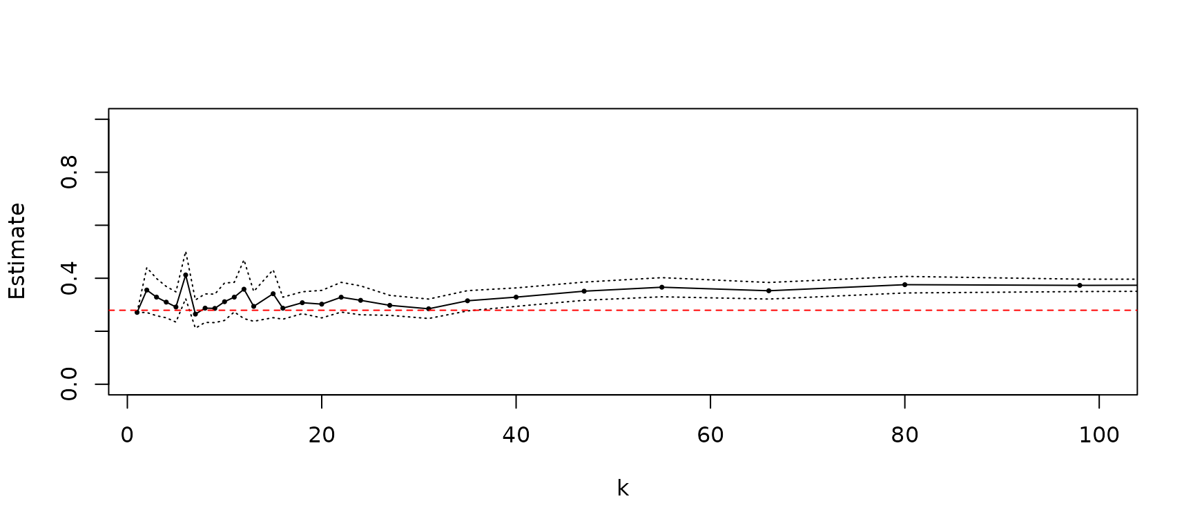
Similarly, we can produce this plots with the option plot=T. The dashed line in blue gives the estimate for k = 10.

estimate     <-  piCP(path,alphae,plot=T)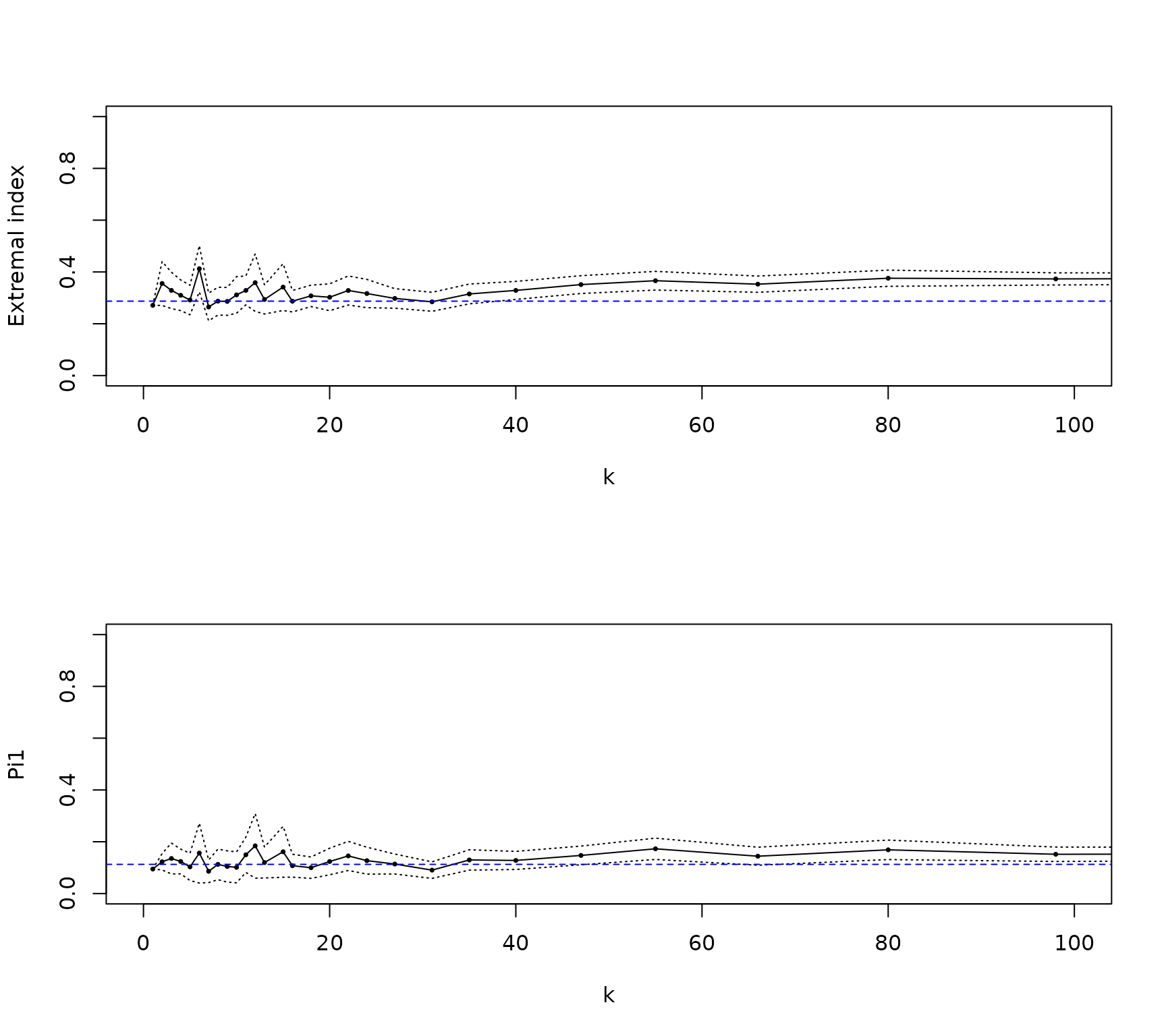

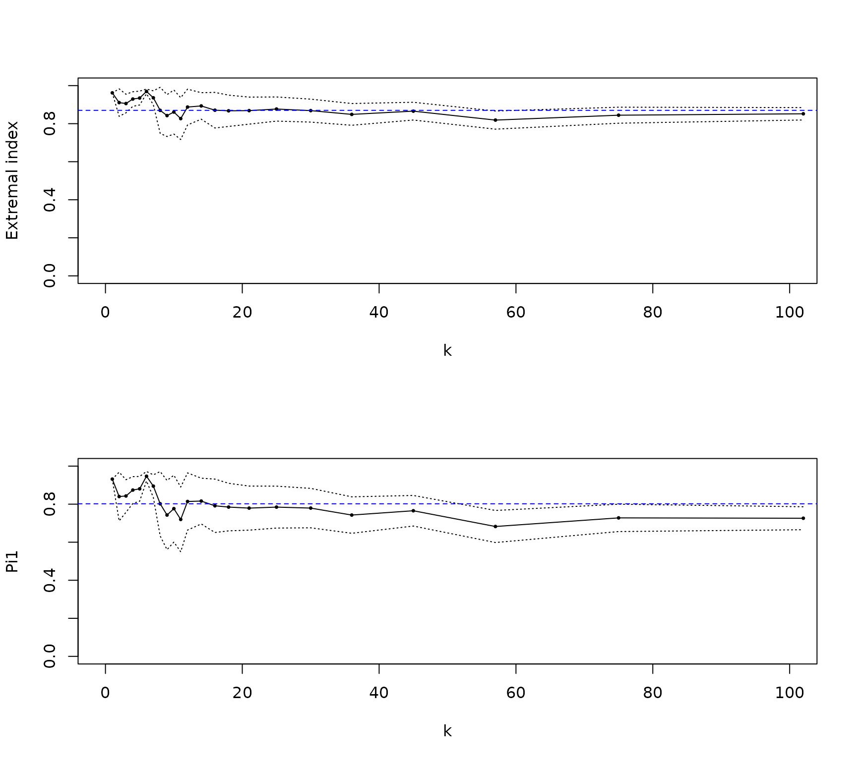
Finally, recall the rainfall data set that we presented in the tail index analysis. We can now apply our method to this data set.

path         <- rainfall$BREST[rainfall$SEASON=="SPRING"]
alphae       <- 1/alphaestimator(path,k1=150)$xi 
estimate     <- piCP(path,alphae,plot=T)

References

Davis, Richard A., and Thomas Mikosch. 2009. “The extremogram: A correlogram for extreme events.” Bernoulli 15 (4): 977–1009. https://doi.org/10.3150/09-BEJ213.

Kulik, R., and P. Soulier. 2020. Heavy-Tailed Time Series. Springer.